GW 150914: The first observation of a gravitational wave signal

On September 14, 2015 the two LIGO detectors recorded the first direct observation of gravitational-waves (GWs) passing over the Earth. This is a milestone in physics and the birth of a new field of astronomy. Below we will explore the "sounds" from this event. First, some key facts about the discovery. 

History:

• After formulating his final field equations for general relativity in 1915, Einstein predicted the existence of gravitational waves in 1916.
• The first experimental efforts to directly detect GWs started with Joseph Weber in the 1960s. Along with several other groups who developed "Weber bar" detectors, this effort was joined in the 1970s by laser interferometers (following pioneering work by Rai Weiss, Robert Forward, and others).
• In 2000 LIGO began operations, reaching design sensitivity in 2006. LIGO is funded by the National Science Foundation and managed by Caltech & MIT. The initial LIGO detector was sensitive to only the strongest GW events (which are expected to happen once or twice a century). LIGO was joined by other large-scale interferometers Virgo, GEO 600, and TAMA 300.
• Parallel to the experimental work, a significant effort began in the 1960s to model the inspiral and merger of two compact objects. This involved contributions from analytical models (pencil & paper) and numerical simulations on supercomputers. In 2005 a milestone was reached with the first successful computer simulations of merging black holes. Theoretical models of the signal continue to play a crucial role in detecting GWs.
• In 2010 a major upgrade of LIGO began (the Advanced LIGO project). This upgrade was part of the original vision for LIGO and was completed in 2014. The first observations began in 2015. The upgrade cost $200 million dollars. The total NSF-supported costs for LIGO construction, upgrades, operation, and support to individual researchers has been $1.1 billion. 
• The first detection of gravitational waves occurred on September 14, 2015. This event is called GW150914.

Key facts about GW150914:

• LIGO made the first observation of two black holes merging together.
• The black holes had masses of 29 and 36 times the mass of the sun. They merged to form a single black hole with a mass of 62 solar masses. That black hole remnant spins at a rate of 100 rotations per second.
• An energy equivalent to the mass of three suns was released by the inspiral and merger of these black holes. This energy release happened over a time period of  two-tenths of a second (0.2 sec). During that brief moment, this system released energy at a rate that was 50 times the energy output rate of all the stars in the entire observable universe (3.6 X 10^56 erg/s or the equivalent of 200 solar masses per second).
• This merger of two black holes happened 1.3 billion years ago, when the earth contained only simple multicellular life. Since GWs travel at the same speed as light, this merger occurred about 1.3 billion light years away.
• The event was seen in both LIGO detectors with a time offset of 7 milliseconds (consistent with the time for the GWs to pass from the Livingston, La detector to the one in Hanford, Wa, accounting for the direction in space the waves originated from and the fact that GWs travel at light-speed). 
• The event was found in the data via multiple analysis methods and with high statistical significance. The signal was a strong one. The detector and local environment would randomly cause simultaneous disturbances of this magnitude in both detectors only at a rate of once every 203,000 years.
• The signal is completely consistent with the predictions of general relativity and agrees well with the predictions of numerical calculations that model the merger of two black holes. This is the first time general relativity has been tested in conditions of extremely-strong gravity. General relativity has passed every experimental test to which it has been subjected.

The "big picture:"

• This is first time GWs have been directly detected by instruments on Earth. The detection was unambiguous and thoroughly vetted. (The effect of GWs on the orbital motion of binary neutron stars was previously observed with radio telescopes. The discovery of the first system to show this effect was awarded the Nobel prize in 1993.)
• This is the first time we have observed two black holes collide and merge, forming a single black hole. This is also the first time we have observed stellar mass black holes with such large masses; it is the first stellar-mass black hole binary to be discovered.
• LIGO has made the most precise length measurement ever. The LIGO mirrors moved in response to GW150914 by an amount roughly equal to 1/1000th the diameter of a proton. This measurement is equivalent to measuring the distance to the nearest start (Proxima Centauri, 4.24 light-years away) to within the width of a human hair (and thin hair at that).
• This discovery is important because it represents the birth of a new field of astronomy. We will now be able to "listen" to a class of celestial phenomena that were previously inaccessible to us with electromagnetic astronomy. Every time we have previously observed the universe with new tools, we have discovered entirely new phenomena. 
• Exploring the universe with this new tool and previously developed ones helps us to understand our origins---how everything came to be the way it is. We are also probing how the fundamental laws of nature work. Like the other great works of humankind---Shakespeare, Mozart, da Vinci, and countless other artists and scholars---the process of discovery and understanding enriches our lives. It inspires the next generation of scientists (and helps employ the current generation). This discovery illustrates to society that the natural world is understandable via rational investigations. It is an amazing discovery---originating from the thoughts of Einstein 100 years ago, and brought to fruition by the hard work of thousands of scientists since then.

More information about the discovery can be found here:

• Caltech Announcement Site
• Caltech Media Assets Site with links to press conference recording and other videos/animations
• LIGO Lab Detection Site
• MIT Announcement Site
• LIGO Open Science Center (LOSC) data release on GW150914
• LSC Science Summaries (including a summary of the detection paper). That page also links to a general FAQ about LIGO.
• The discovery paper in Physical Review Letters, and the Physics Viewpoint article by Emanuele Berti explaining the discovery.
• NSF detection press conference; (part 2 has additional Q&A).
• Caltech post-detection panel discussion, Ripples in Spacetime

A beautiful illustration of GW150914 is seen in this numerical simulation by the Simulating eXtreme Spacetimes (SXS) numerical relativity group:

This video shows the event horizons of the two black holes as they merge into one. The colored spots on the horizons indicate the spin axes of the black holes (which change orientation due to spin-coupling interactions that are predicted by general relativity). The colored lines illustrate the orbital paths. The horizons eventually merge and form a single rotating black hole. The surface below the event horizons indicates the curvature of space. The coloring of the surface indicates the "curvature of time"---time passes more slowly near the black holes (redder color) than farther away. The distant ripples in the surface illustrate the GWs emitted by the system. (These ripples and the curvature of space happen in 3-dimensions; only a 2-dimensional representation can be easily displayed.) At the very bottom we see the GW signal being traced out as the merger progresses.

You can find more GW150914 animations by the SXS group at their youtube channel or on their website. [The image at the top of this page is a frame from their animation.]

And now for the sounds...
​

"Sound" from GW150914

Below we see an animation with sound produced by the LIGO collaboration. The curve shows the whitened GW signal (strain vs. time) seen in each LIGO detector. (This is explained below.) The orange and blue colored regions above the curves show the time-frequency evolution of the signal. The frequency increases very rapidly with time near the merger. The intensity of the color indicates the increasing strength of the signal. This is the characteristic "chirp" behavior of the gravitational-waves from merging black holes.

A sound accompanies the animation. This sound is a conversion of the GW signal to an audio representation. (This analogy is explored throughout this site.) The sound first repeats twice at the actual frequency of the GW signal. (The sound is at low frequencies and may be difficult to hear---it will sound better with headphones or good speakers.) The sound then repeats two more times, but artificially shifted higher in frequency to make it more audible. This sequence of sounds then repeats again (real frequency twice, shifted frequency twice).

This "sound" represents the start of a new way of perceiving cosmic events. We were previously "deaf" to the universe, but not any longer.
​

Exploring the signal and the noise

Let's examine in more detail the signal that LIGO observed. This will be a slightly more advanced discussion than what was presented above. [You can download the data shown below from the GW150914 data release page at the LIGO Open Science Center (LOSC).] 

The key observable for LIGO is the strain, the fractional difference between the change in the lengths of the two arms of the interferometer. [The GW causes a length change in each "arm" of a GW detector; the interferometer signal is the difference between the length changes in the two separate arms. Dividing this difference by the 4 km length of the arms gives the strain h(t).] The GW that was detected produced a peak strain of 10^(-21). This is a very tiny signal. Other influences in the environment or the detector itself will regularly cause much larger strains. Even for a strong source like GW150914, the signal will not be readily apparent by looking at the data (as we will see below). Instead, one must filter the data in some way to make the signal visible. (This is done after one has searched through all the data and identified a strong candidate signal.)

Here is what the "raw" strain data looks like from the two detectors (Hanford/H1 in red and Livingston/L1 in blue). We show the data taken from the LOSC sampled at a rate of 4096 Hz. Here is a 32 second stretch of data with GW150914 at t = 0 s, followed by several zoom-ins near the location of the signal from GW150914. Sounds of the strain data follow the plots.

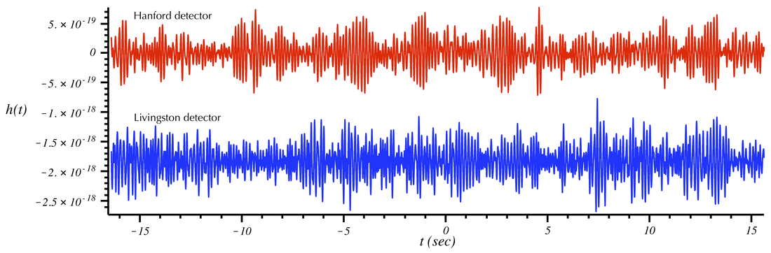
Gravitational-wave strain data from the Hanford (top/red) and Livingston (bottom/blue) LIGO detectors. A 32-second time window centered on the GW150914 signal is shown. [Data here and below from LOSC. There is a very low-frequency oscillation that causes the Livingston strain to be offset from 0 during this stretch of data. These low-frequency modulations do not affect the data analysis.]

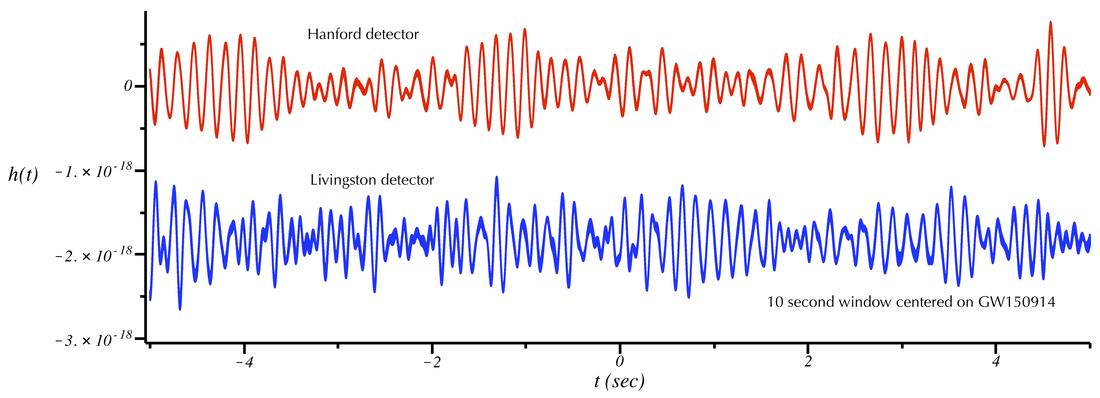
Same as above, but showing a 10 second time window around GW150914.

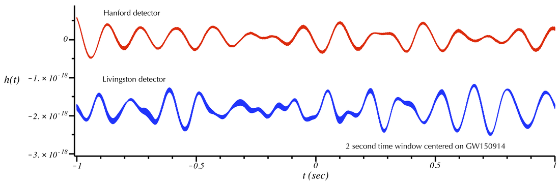
Same as above, but now showing a 2-second time window. The oscillations seen here and in the above plots are low-frequency detector noise. No signal is visible by eye.

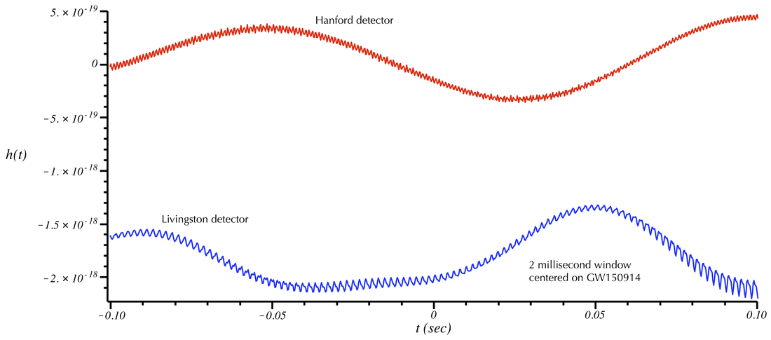
Zooming-in still more to a 2-millisecond time window. The small-oscillations visible here have amplitudes ~10^(-19). This is 100 times larger than the gravitational wave signal. GW150914 fills much of this time window, but there is no way to see it without filtering the data. One can easily verify that the small-scale oscillations on the blue curve have a frequency ~500 Hz. This is above the frequency of GW150914 and corresponds to the fundamental vibration mode of the test mass suspensions. GW150914 contains frequency components in the range of 20 Hz to 300 Hz.

There is a signal in the above sounds and plots, but it is not possible to hear or see it without manipulating the data a bit. If the data is filtered to remove frequency components where the noise is large, then a signal emerges as shown in the following plots. [The filtering process removes strong instrumental "noise lines" in the data as well as frequency components below 35 Hz and above 350 Hz. This process is discussed at this LOSC tutorial.]

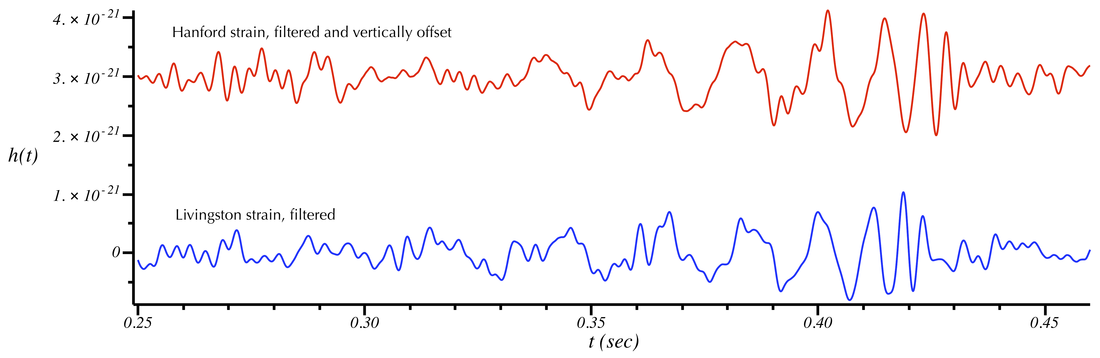
Filtered Hanford and Livingston strain. Frequency components outside the band of GW150914 have been removed. A signal now becomes apparent. The Hanford signal is delayed by about 7 milliseconds due to the time for the gravitational-wave to propagate between the detectors. (The Livingston detector received the signal first.)

Here are the sounds roughly corresponding to the above, and taken from the audio files at the LOSC GW150914 data release. Note that the sounds last for about 4 seconds and are longer than the data range in the above plot. The filtering applied to the data used to generate the sounds is also slightly different from what's described above. [The bandpass range is a bit different and a whitening filter has been applied. See the above link for details.] The first set of sounds are at the actual frequencies found in the data. The second set shifts the sounds upwards in frequency by 400 Hz. The former can only be heard well with headphones or real speakers. The latter can be heard on laptop speakers.

The consistency of the above Hanford/Livingston signals can be seen by plotting them on top of each other (and flipping the sign of the Hanford signal). [Because there is a roughly 90 degree difference in the relative orientation of the two LIGO sites, this introduces a change in the detector response between the two sites that is equivalent to multiplication by a minus sign.] The result is the following: 

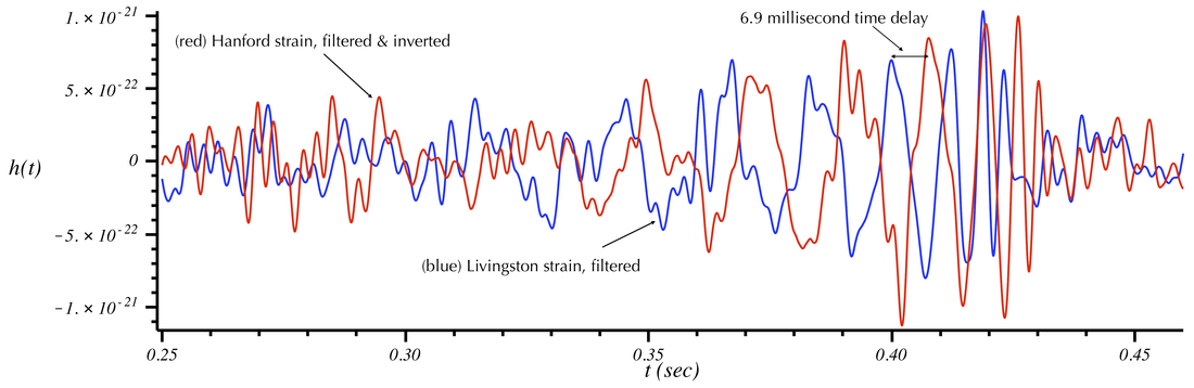
Same as above plot, with Hanford signal inverted and shown on top of the Livingston signal. (As in the last plot, this is the filtered data.)

Notice that there is a clear time offset between several peaks due to the lightspeed propagation time of the GW from Livingston to Hanford. If we artificially shift the Hanford signal, the peaks will align:

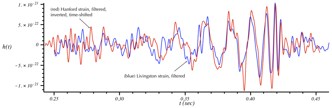
Same as above but with the Hanford data shifted backwards in time by 6.9 milliseconds.

This demonstrates that filtering of the data produces two strong signals time-shifted by an amount consistent with the light-speed travel time between detectors. Additionally, the signal was shown to be consistent with theoretical models of merging black holes. Note that the signals were not discovered via this filtering process. But once found, the filters described above can be used to make the signal apparent. (To initially identify the signal and make a first estimate of its characteristics,  a large number of template signals is compared with the data in both detectors.)

Once the signal is identified, a refined analysis attempts to determine the model parameters (masses, spins, sky location, etc) that are a best-fit to the data. This best-fit model is shown below (as projected into the Hanford detector), followed by its "sound" (in stereo).

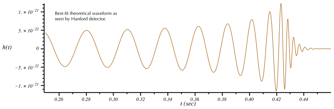
Best-fit model for the gravitational wave signal as would be seen in the Hanford detector. This signal is consistent with numerical simulations of the merger of two black holes as predicted by general relativity. The black holes have masses 29 and 36 times the mass of the sun.

To visually compare the above best-fit model with the filtered data above, the same filter must also be applied to the model. The next plot shows this, with the filtered model superimposed on the unfiltered version shown above. The sound corresponding to the filtered best-fit model follows the plot.

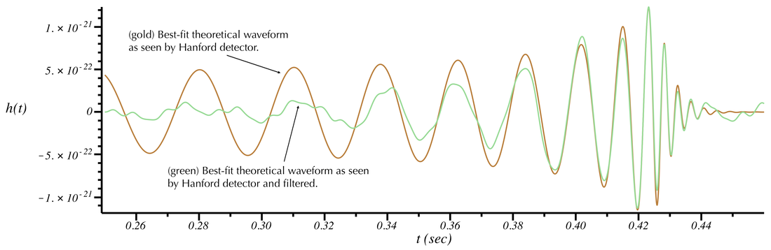
Best-fit model above along with filtered version of the best-fit (as seen by the Hanford detector). This adjusts the model to account for the detector's sensitivity at different frequencies.

Looking at the above plot, one can easily tell from the peak-to-peak distance that the frequency of the best-fit waveform near t=0.3 s is close to 30 Hz. Near the merger it is closer to 150 Hz and increases to ~300 Hz during the ringdown. The green curve adjusts the best-fit model to incorporate those frequencies that were modified by the filtering applied to the data. (For example, note that the amplitude of the green curve is suppressed at low frequencies, but matches the unfiltered data at high frequencies close to merger.) With this filtering applied, we can now compare the best-fit model to the filtered data:

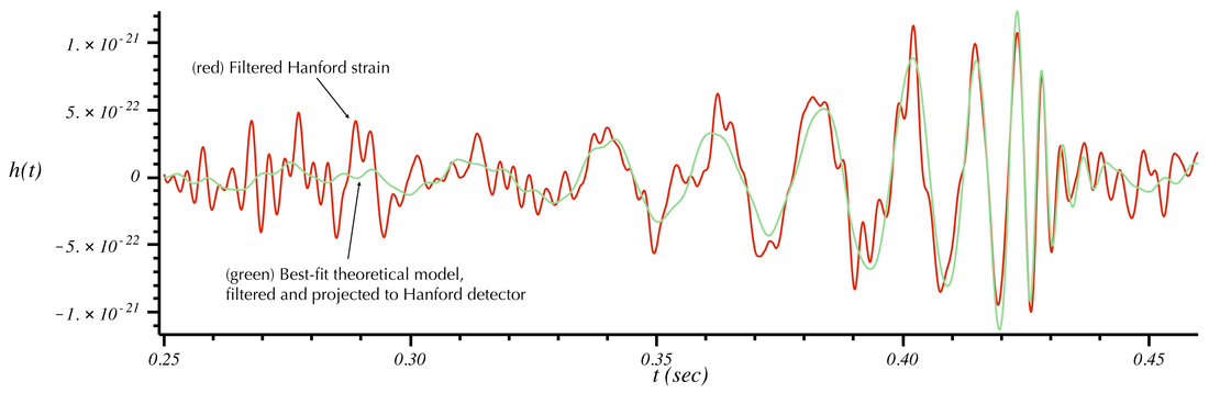
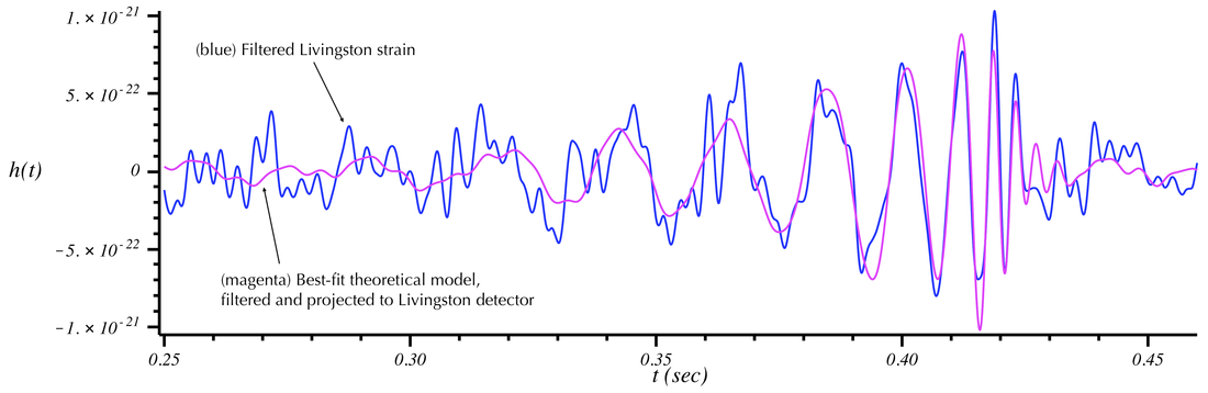
Comparison of filtered strain data (Hanford/red and Livingston/blue) with filtered best-fit theoretical model as viewed by each detector (red/magenta). The location of the peaks overlap nicely (especially near merger), indicating strong agreement between the data and the model.

​Look at that beautiful agreement. Einstein was right...again!

Stereo sounds and the sky position of GW150914

Unlike an optical telescope, a single LIGO detector can say very little about where on the sky a gravitational wave is coming from. This is analogous to the relationship between our own hearing and sight. A single eye is very good at pinpointing the direction of a small flash; a single ear is not good at finding the direction of a short, sharp sound. But two ears are better one---and because we have two, humans have some ability to determine the direction from which a sound originates---but only to a crude accuracy (of order 1 to 15 degrees depending on the direction of the sound). One of the main ways we are able to determine sound direction is via the time difference between the sound recorded by our left and right ears. This difference is at most about 0.6 milliseconds (although shorter time differences can be perceived). This same trick is used by gravitational-wave detectors to localize the origin of the gravitational wave. (Like our ears, GW detectors also use information about the relative "loudness" or amplitude of the waves and the phase information contained in the signals observed in each detector. Here we will focus on the effect of the time difference. You can learn more about how our ears determine sound direction at the wikipedia articles for sound localization and interaural time difference. )

The two LIGO detectors are part of a developing global network of gravitational-wave detectors. At the time GW150914 was detected, only the two LIGO detectors were in an observational mode. Along with the smaller GEO600 detector in Germany, LIGO will soon be joined by an upgraded Virgo detector in Italy. Later this decade and in the early 2020s, these detectors will be joined by the Kagra detector in Japan and a third LIGO detector in India. The map below shows the location of these observatories. (There are also proposals for a detector in Australia.)  

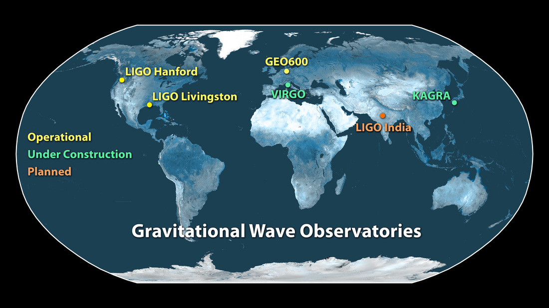
Map showing the location of current and future gravitational-wave detectors. Image credit: LIGO.

The two LIGO detectors are separated by about 3000 km. It takes gravitational waves (which travel at the same speed as light) a maximum of 10 milliseconds to propagate from one detector to the other. This would be the time difference if the waves were traveling parallel to a line connecting the two detectors. If the waves were traveling perpendicular to this line, the time difference would be zero. A wave coming from an arbitrary direction will register a time difference inbetween these values and thus provides some information about the direction in the sky the waves originate from. For GW150914, a time difference of about 7 milliseconds was registered between the two detectors. That information, along with amplitude and phase information contained in the two signals, allowed LIGO to make an estimate of the sky position of GW150914. This is shown in the following image:

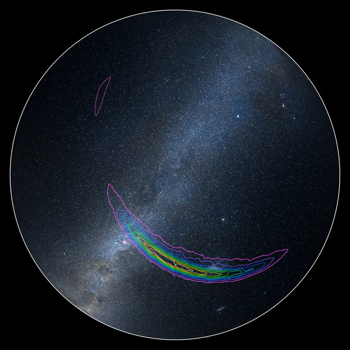
Estimated sky position of GW150914. The colored lines show contours of different degrees of certainty. For example, the purple contours represent the area on the sky where GW150914 is located with 90% confidence. The inner yellow lines represent the region of 10% confidence. The background shows an optical image of the Milky Way. A nearby satellite galaxy of the Milky Way---the Large Magellanic Cloud---lies underneath the banana-shaped contours. Image credit: LIGO/Axel Mellinger.

Because only the two LIGO detectors recorded a signal from GW150914, the 7 millisecond time delay allowed the origin point of the waves to be localized to a thick ring-shaped area on the sky. This is essentially the same process as triangulation or trilateration. This is used by GPS satellites or cell phone towers to determine your location. With only two detectors, the source of a signal can only be located to a ring-shaped region (the intersection of two spheres). A third detector narrows this down to two points on the ring (since a ring intersects a sphere at two distinct points). [See this website for a nice animation showing how this works.] In the case of the two LIGO detectors, additional information from the amplitude of the waves allowed further localization of GW150914 to a segment of a ring shown above. (The small purple region in the upper-left of the image represents another part of the ring that cannot be fully excluded with 90% confidence.) This region has an area of about 600 square degrees. This represents about 1.5% of the total area of the sky. While this may sound small, this is actually a very big region, especially in comparison to the capabilities of optical telescopes. The full moon spans an area of 0.2 square degrees, so 600 square degrees is an area equivalent to 3000 full moons---a very big sky area indeed. Once additional gravitational-wave detectors come on-line (Virgo, Kagra, LIGO-India), our ability to localize signals will improve significantly. 

For GW150914 the primary localization comes from the 7 millisecond time difference between the signals registered in each LIGO detector. Let's explore the "sound" of this time difference. Below we show the signals from the two detectors (Hanford/H1 in red; Livingston/L1 in blue). These signals were extracted using a different technique from those shown in the above section. [An algorithm called coherent WaveBurst was used, which makes minimal assumptions about the shape of the signal. Like the above, the extracted signals were filtered (or whitened in this case) in a particular way to account for the varying frequency response of the detector. The signal is completely consistent with that shown above, but differs slightly in the details because of the different data analysis techniques that were used. The data shown here is taken from the LOSC GW150914 data release website and is discussed further in this paper.]  

The first plot below shows the actual times that the two signals arrive in each detector. In the second plot we artificially time-shifted the Hanford signal to 6.9 milliseconds earlier. Notice that now the peaks line up. This is how we can determine the time delay. The precise duration of this delay provides information about the direction the signal came from. Below the two plots are stereo sounds, with Hanford in the left channel and Livingston in the right channel. (The frequency or duration of the sound has not been altered.) Listen to the sounds with headphones and see if you can perceive the Livingston sound hitting your right ear first, followed by the Hanford sound in your left ear.

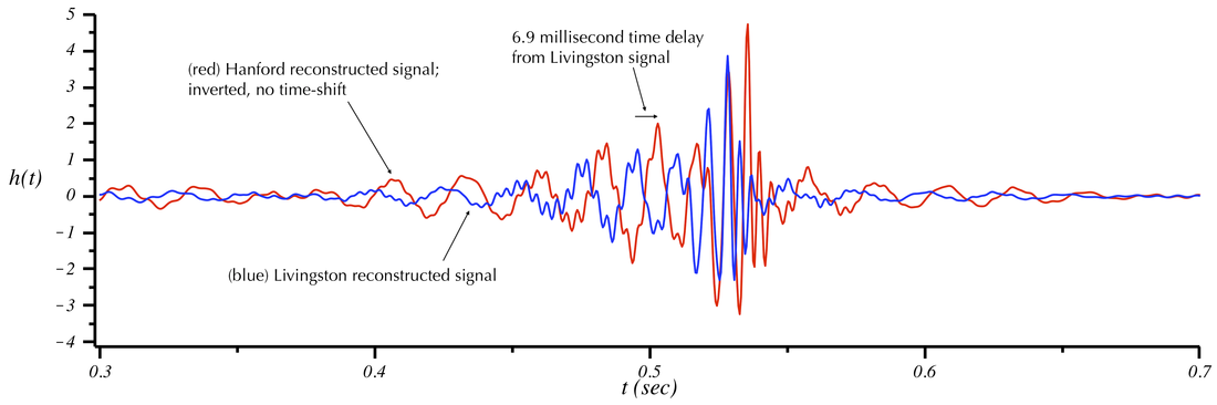
Reconstructed signals from GW150914 as seen in the Hanford (red) and Livingston detectors. The Hanford signal is inverted to account for the relative orientations of the two detectors. The actual time-of-arrivals are shown in this plot. The y-axis is normalized differently from other plots on this page. The scaling represents the number of standard deviations away from the noise level in the detector.

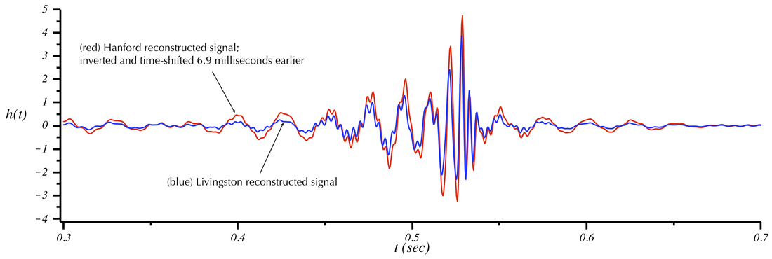
Same as above except the Hanford signal has been shifted 6.9 milliseconds earlier in time. Notice that the peaks line up perfectly.

Listen to the above two sounds and compare them. Can you hear a slight offset between your two ears in the first sound?

It is very difficult to hear the difference, but it is perceptible. To make the time difference more apparent, let's now induce an additional time off-set in the Hanford signal. The actual 6.9 millisecond offset is the time it takes the signal to propagate from the Livingston detector to the Hanford one (along a particular direction direction in space). Suppose the two detectors were separated by a much larger distance than 3000 km. There would be an even larger time delay between the signals detected at the two sites. To explore this, we have added in the first plot below an additional 32 millisecond time delay to the Hanford signal. This corresponds to two detectors on opposite sides of the Earth (so the signal must propagate a distance of two Earth radii or 12,740 km after it encounters the first detector). In the second plot we show the case when this separation is increased to two Earth diameters. Play the sounds below the plots---you should be able to clearly hear the time delay between the two signals. It should seem like the signal is passing from your right ear to your left ear---corresponding to a signal coming from your right.

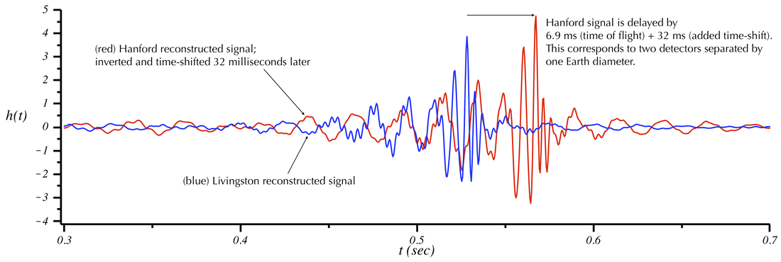
Similar to the above two plots except an additional time-shift has been added to the Hanford signal (corresponding to two detectors on opposite sides of the Earth).

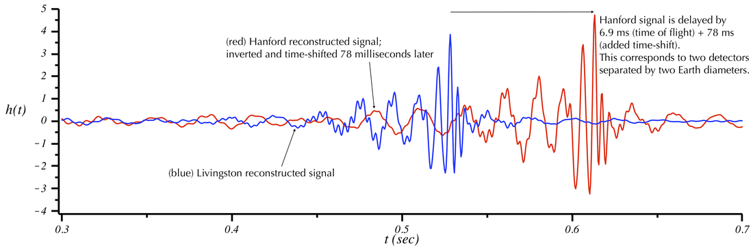
Same as above except a time-shift of 78 milliseconds was added to the Hanford signal corresponding to two detectors separated by two Earth diameters.

In the above two sounds you can clearly hear the time offset in the two signals. The right speaker plays the sound first, followed by the left speaker. You perceive this as a sound coming from the right and moving leftwards. In a similar way, the time delay between the signals recorded in two or more gravitational-wave detectors provides information on the direction of the astrophysical event that produced the waves.